A Quick Start to pyPetal
pyPetal is a pipeline that contains 7 modules, each of which can be used optionally, and having its own parameters. A more in-depth description of the entire pipeline can be found in the API section.
The 7 modules available are:
DRW (Damped Random Walk)-based outlier rejection
Detrending
pyCCF
pyZDCF
PyROA
JAVELIN
Weighting
Here, we’ll describe the five main modules that can be used (DRW Rejection, pyCCF, pyZDCF, and JAVELIN). Detrending and weighting (as well as the other modules) are decsribed in detail in further tutorials and the API.
Main Arguments
pyPetal only takes a few required inputs to run, while all of the modules and their parameters are optional. The required inputs are:
output_dir: The directory where the output files will be saved.arg2: Either a list of paths to the input light curves, or an array with the light curves themselves.
Note
The first light curve will be assumed to be the continuum light curve.
Note
All light curve files must be in the same directory and have the same format.
There are a few optional general arguments as well:
line_names: A list of names corresponding to the light curves.verbose: If the progress (text only) should be printed.plot: If figures should be displayed throughout the run.time_unit: The unit of the time data for the input light curves.lc_unit: The units of the input light curves.lag_bounds: The bounds to search for the lag between two light curves.threads: The number of threads to use for multiprocessing.
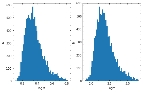
DRW Rejection
The Damped Random Walk (DRW) is a popular model used to describe the variability of AGN data, with a power spectral density (PSD):
\(P(f) = \frac{4 \sigma_{\rm DRW}^2 \tau_{\rm DRW} }{1 + (2\pi f \tau_{\rm DRW})^2}\)
with two parameters: \(\sigma_{\rm DRW}\), \(\tau_{\rm DRW}\)
We can fit an arbitrary light curve (or a set of them) to a DRW model using the Gaussian process solver celerite with MCMC algorithm emcee. In this example, we’ll use PETL to fit each light curve to a DRW model and reject all points that are more than \(3\sigma\) from the mean of the DRW fit.
[1]:
import pypetal.pipeline as pl

main_dir = 'pypetal/examples/dat/javelin_'

filenames = [ main_dir + 'continuum.dat', main_dir + 'yelm.dat', main_dir + 'zing.dat' ]
output_dir = 'quickstart_output/'
line_names = ['Continuum', 'H-alpha', 'H-beta']
[2]:
res = pl.run_pipeline( output_dir, filenames, line_names,
                       run_drw_rej=True,
                       verbose=True,
                       plot=True,
                       file_fmt='ascii',
                       time_unit='d',
                       lc_unit='mag')
Performing DRW rejection
------------------------
jitter: True
nsig: 3
nwalker: 100
nburn: 300
nchain: 1000
clip: array
reject_data: [ True False False]
use_for_javelin: False
------------------------

This will output a number of plots (like shown above) and diagnostic information in the specified output_dir. In particular, the light curves will be saved in CSV format along with the DRW rejection masks in the light_curves subdirectory. The processed_lcs subdirectory will contain the light curves with the rejected points removed.
By default, only the first (i.e. continuum) will be fit to a DRW and have points rejected, though this can be specified in the reject_data argument.
pyCCF
Now, we can utilize the pyCCF code to get the (interpolated) cross-correlation function between the continuum and the two light curves. To do this, we only need to specify run_pyccf=True in run_pipeline.
[3]:
res = pl.run_pipeline( output_dir, filenames, line_names,
                       run_pyccf=True,
                       verbose=True,
                       plot=True,
                       file_fmt='ascii',
                       time_unit='d',
                       lc_unit='mag',
                       threads=45)
Running pyCCF
-----------------
lag_bounds: [[-1976.98849, 1976.98849], [-1976.98849, 1976.98849]]
interp: 2.0000000001
nsim: 3000
mcmode: 0
sigmode: 0.2
thres: 0.8
nbin: 50
-----------------

Failed centroids:  0
Failed peaks:  0
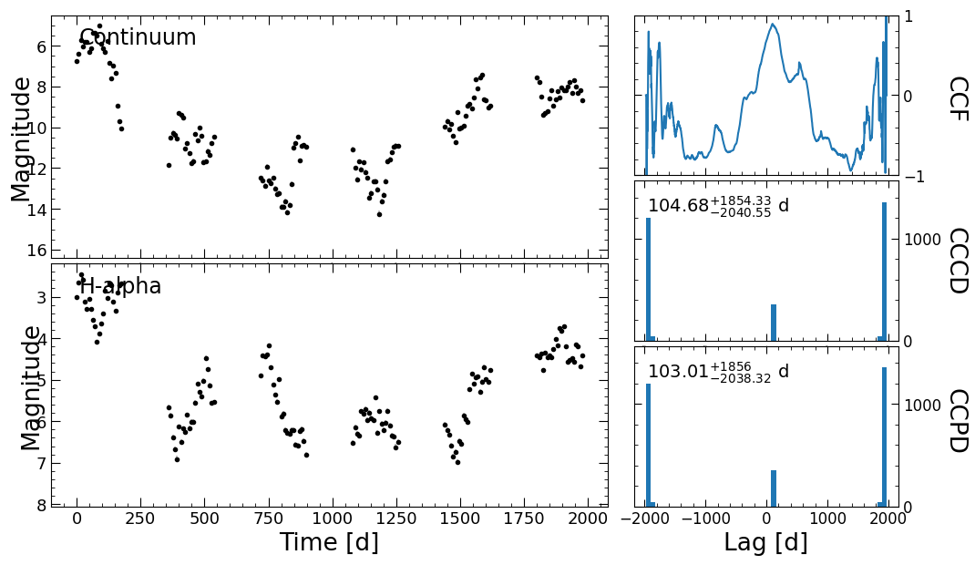
Failed centroids:  0
Failed peaks:  0
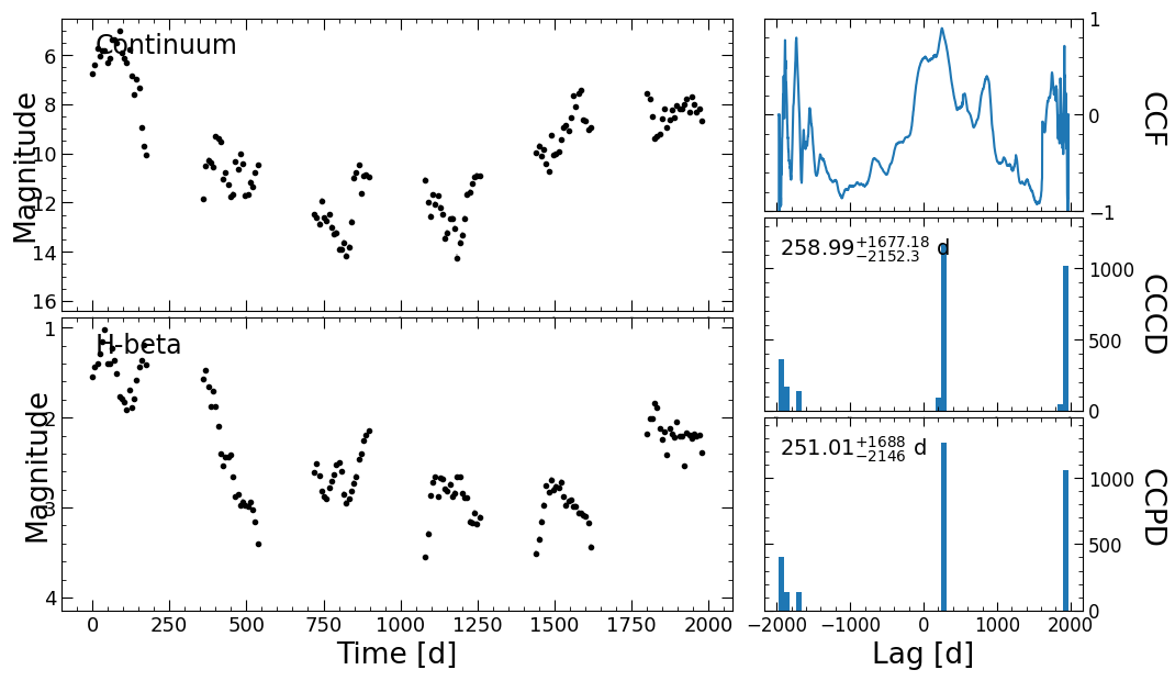
This produced two plots showing the continuum of each of the lines, the cross-correlation function (CCF), the cross-correlation centroid distribution (CCCD), and the cross-correlation peak distribution (CCPD).
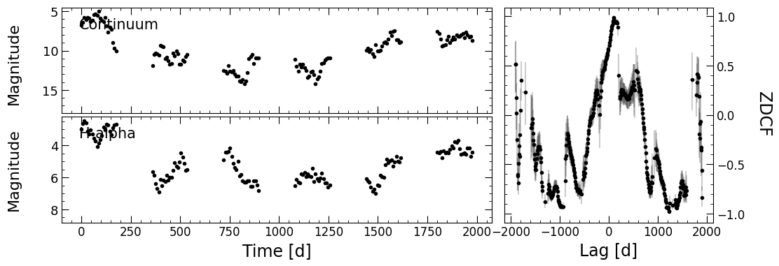
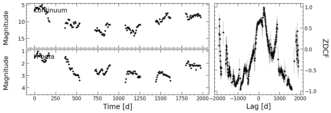
pyZDCF
The next module in pyPetal is the pyZDCF module, which computes the Z-transformed Discrete Corrrelation Function between the continuum and each of the two lines. Similar to pyCCF, we only need to specify run_pyzdcf=True in run_pipeline.
[4]:
res = pl.run_pipeline( output_dir, filenames, line_names,
                       run_pyzdcf=True,
                       verbose=True,
                       plot=True,
                       file_fmt='ascii',
                       time_unit='d',
                       lc_unit='mag')
Running pyZDCF
----------------------
nsim: 1000
minpts: 0
uniform_sampling: False
omit_zero_lags: True
sparse: auto
prefix: zdcf
run_plike: False
plike_dir: None
----------------------
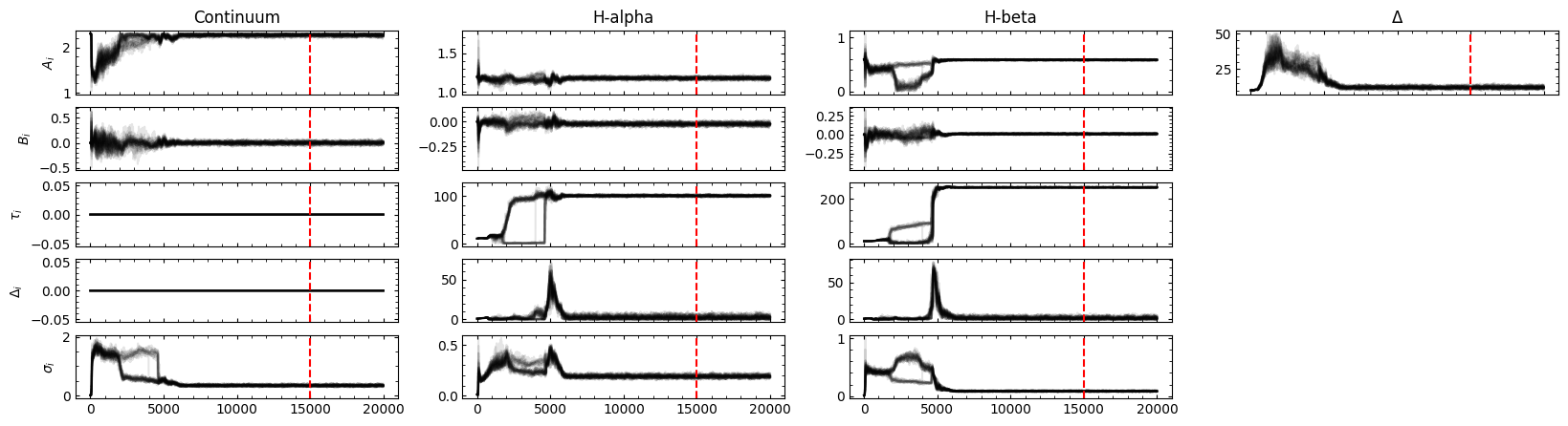
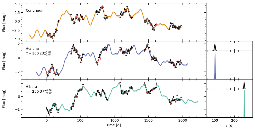
PyROA
The next module in pyPetal uses the PyROA code, which finds and models the lag between two (or more) light curves using the running optimal average (ROA) technique. For more information, see the PyROA tutorial and the original PyROA code (and references therein).
To run this module, set run_pyroa=True in run_pipeline.
By default, this will fit all lines to the continuum separately in one run. The light curves saved in PyROA’s format will be stored in the pyroa_lcs subdorectory in the output_dir. The diagnostic information and plots output from PyROA will be saved in the pyroa subdorectory in the output_dir.
[5]:
res = pl.run_pipeline( output_dir, filenames, line_names,
                       run_pyroa=True,
                       verbose=True,
                       plot=True,
                       file_fmt='ascii',
                       time_unit='d',
                       lc_unit='mag')
Running PyROA
----------------
nburn: 15000
nchain: 20000
init_tau: [10.0, 10.0]
subtract_mean: True
div_mean: False
add_var: True
delay_dist: True
psi_types: ['Gaussian', 'Gaussian']
together: True
objname: pyroa
----------------
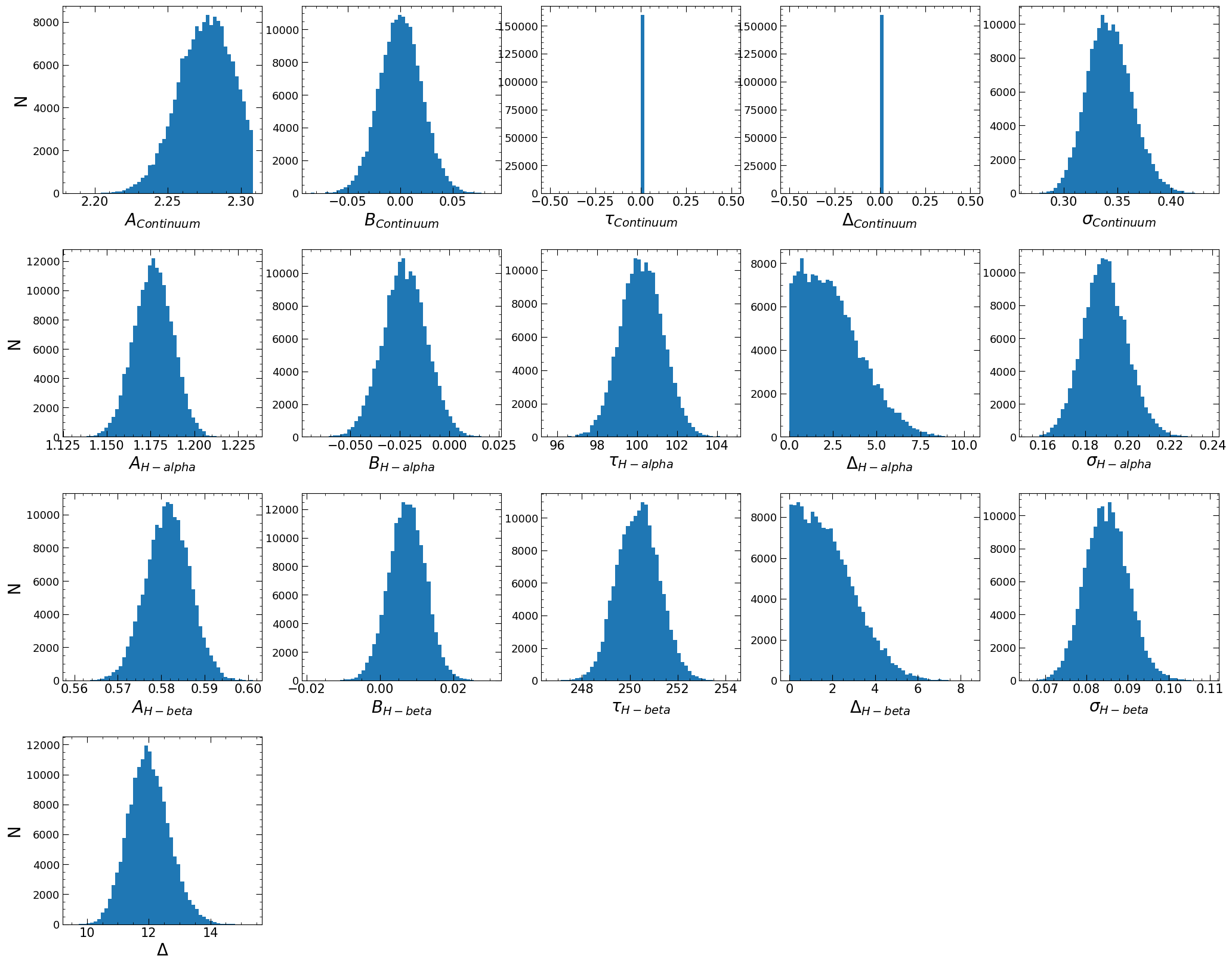
Initial Parameter Values
A0 B0 σ0 A1 B1 τ1 Δ1 σ1 A2 B2 τ2 Δ2 σ2 Δ
------- ----------- ---- ------- ----------- ---- ---- ---- ------ ---------- ---- ---- ---- ---
2.30824 7.53021e-16 0.01 1.19302 4.11909e-16 10 1 0.01 0.5882 3.6042e-16 10 1 0.01 10
NWalkers=32
100%|██████████| 20000/20000 [43:15<00:00, 7.71it/s]
Filter: Continuum
Mean Delay, error: 0.00 (fixed)
Filter: H-alpha
Mean Delay, error:  100.23119  (+   1.04209 -   1.07512)
Filter: H-beta
Mean Delay, error:  250.36897  (+   0.88959 -   0.86571)


Best Fit Parameters
     A0           B0        σ0       A1          B1       τ1       Δ1        σ1        A2          B2       τ2       Δ2        σ2        Δ
-------  -----------  --------  -------  ----------  -------  -------  --------  --------  ----------  -------  -------  --------  -------
2.27618  0.000371373  0.341979  1.17664  -0.0226682  100.231  2.24521  0.189107  0.581586  0.00742638  250.369  1.65488  0.084886  11.9802

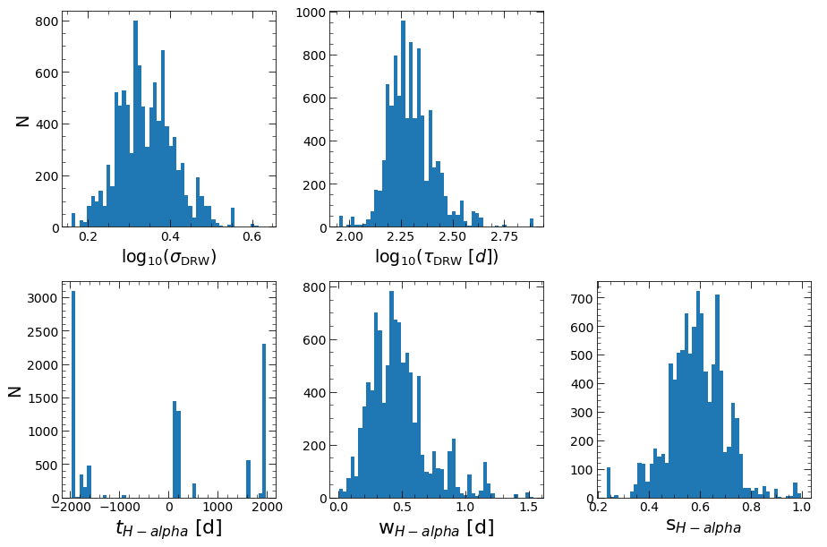
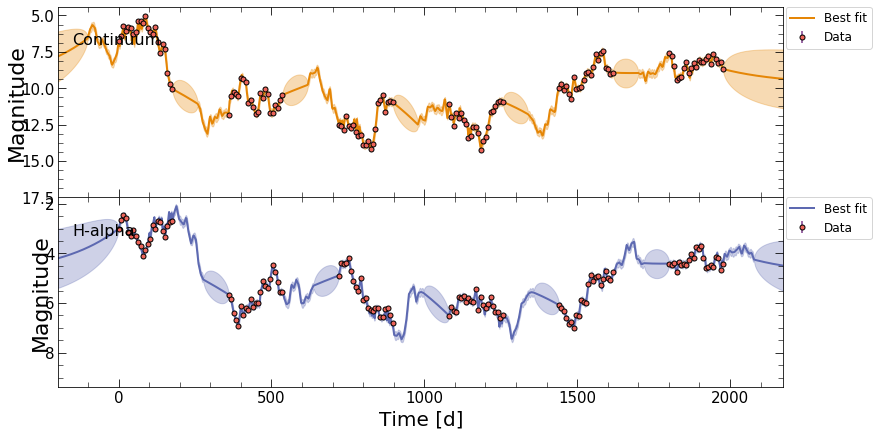
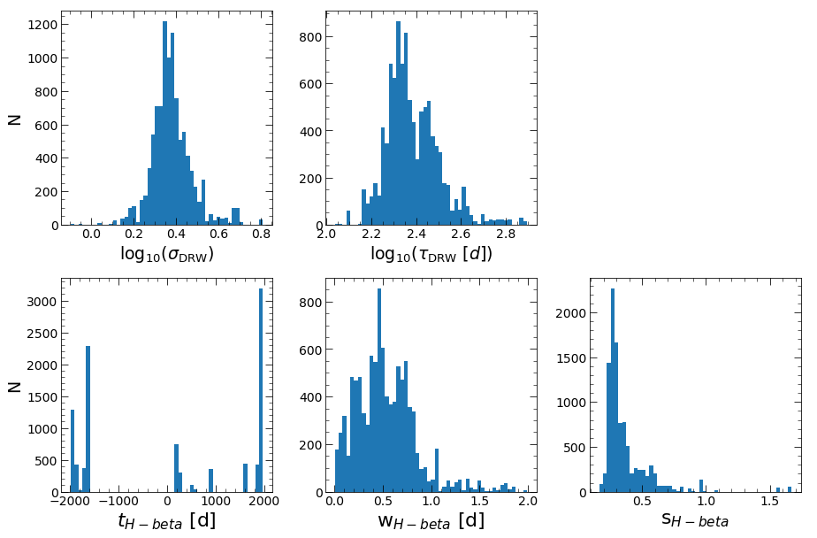
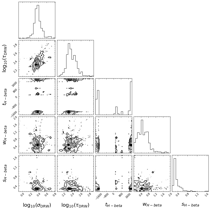
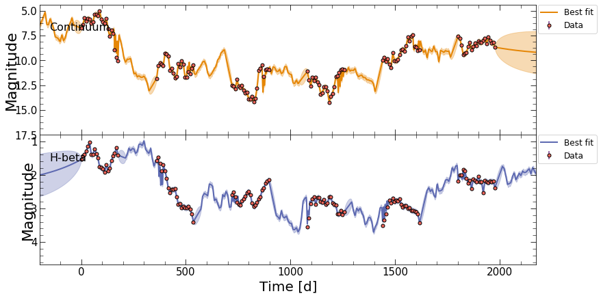
JAVELIN
The final module in pyPetal uses the JAVELIN code, which finds the lag between the continuum and multiple lines by interpolating with a fitted Damped Random Walk (DRW) model, convolved with a moving tophat function.
JAVELIN is unique in that it requires a separate version of Python (<3.0), and hence a separate package. This package, pypetal-jav, can be installed through pip, but must be used in a Python 2 environment.
To run this module, we can use the run_pipeline function in pypetal_jav.pipeline. This requires the name of the output_dir from the original pyPetal run, and the line names.
This will fit each pair of continnum and line light curves to the DRW+tophat model, and output a number of plots and diagnostic information in each line’s subdirectory in the output_dir.
[2]:
#Assuming we are now in the Python 2 environment with pypetal-jav installed
import pypetal_jav.pipeline as plj

main_dir = 'pypetal/examples/dat/javelin_'

filenames = [ main_dir + 'continuum.dat', main_dir + 'yelm.dat', main_dir + 'zing.dat' ]
output_dir = 'quickstart_ouput/'
line_names = ['Continuum', 'H-alpha', 'H-beta']

res = plj.run_pipeline( output_dir, line_names,
                       verbose=True,
                       plot=True,
                       file_fmt='ascii',
                       time_unit='d',
                       lc_unit='mag',
                       threads=45)
Running JAVELIN
--------------------
rm_type: spec
lagtobaseline: 0.3
laglimit: [[-1976.98849, 1976.98849], [-1976.98849, 1976.98849]]
fixed: True
p_fix: True
subtract_mean: True
nwalker: 100
nburn: 100
nchain: 100
output_chains: True
output_burn: True
output_logp: True
nbin: 50
metric: med
together: False
--------------------

start burn-in
nburn: 100 nwalkers: 100 --> number of burn-in iterations: 10000
burn-in finished
save burn-in chains to /home/stone28/pypetal/quickstart_ouput/H-alpha/javelin/burn_cont.txt
start sampling
sampling finished
acceptance fractions for all walkers are
0.69 0.68 0.67 0.70 0.67 0.72 0.65 0.73 0.66 0.74 0.77 0.70 0.67 0.71 0.73 0.71 0.67 0.73 0.79 0.65 0.73 0.65 0.72 0.69 0.62 0.68 0.63 0.67 0.66 0.72 0.62 0.73 0.70 0.75 0.64 0.68 0.66 0.74 0.64 0.63 0.79 0.68 0.73 0.70 0.69 0.72 0.70 0.68 0.71 0.65 0.75 0.75 0.59 0.71 0.75 0.69 0.69 0.74 0.77 0.70 0.73 0.63 0.77 0.68 0.74 0.77 0.73 0.69 0.79 0.74 0.66 0.74 0.65 0.72 0.69 0.75 0.71 0.65 0.66 0.74 0.73 0.71 0.79 0.70 0.67 0.79 0.75 0.62 0.69 0.78 0.72 0.65 0.63 0.73 0.68 0.59 0.63 0.81 0.68 0.76
save MCMC chains to /home/stone28/pypetal/quickstart_ouput/H-alpha/javelin/chain_cont.txt
save logp of MCMC chains to /home/stone28/pypetal/quickstart_ouput/H-alpha/javelin/logp_cont.txt
HPD of sigma
low:    1.742 med    2.131 hig    2.931
HPD of tau
low:  135.553 med  207.090 hig  387.869
run parallel chains of number 45
start burn-in
using priors on sigma and tau from continuum fitting
[[  1.742 135.553]
 [  2.131 207.09 ]
 [  2.931 387.869]]
penalize lags longer than 0.30 of the baseline
nburn: 100 nwalkers: 100 --> number of burn-in iterations: 10000
burn-in finished
save burn-in chains to /home/stone28/pypetal/quickstart_ouput/H-alpha/javelin/burn_rmap.txt
start sampling
sampling finished
acceptance fractions are
0.08 0.02 0.00 0.09 0.06 0.04 0.09 0.09 0.03 0.02 0.12 0.02 0.15 0.07 0.06 0.03 0.06 0.07 0.03 0.10 0.02 0.08 0.06 0.12 0.19 0.11 0.10 0.01 0.10 0.07 0.08 0.06 0.09 0.09 0.00 0.13 0.12 0.03 0.10 0.07 0.09 0.02 0.10 0.13 0.12 0.00 0.05 0.09 0.08 0.03 0.03 0.06 0.04 0.07 0.11 0.04 0.05 0.16 0.06 0.09 0.06 0.15 0.06 0.14 0.06 0.03 0.10 0.06 0.05 0.09 0.14 0.04 0.00 0.06 0.10 0.04 0.14 0.02 0.00 0.14 0.09 0.08 0.10 0.00 0.12 0.07 0.04 0.07 0.08 0.09 0.04 0.06 0.14 0.16 0.05 0.09 0.03 0.19 0.06 0.03
save MCMC chains to /home/stone28/pypetal/quickstart_ouput/H-alpha/javelin/chain_rmap.txt
save logp of MCMC chains to /home/stone28/pypetal/quickstart_ouput/H-alpha/javelin/logp_rmap.txt
HPD of sigma
low:    1.879 med    2.167 hig    2.563
HPD of tau
low:  157.070 med  195.034 hig  251.908
HPD of lag_H-alpha
low: -1932.897 med  101.282 hig 1924.632
HPD of wid_H-alpha
low:    0.270 med    0.442 hig    0.648
HPD of scale_H-alpha
low:    0.492 med    0.590 hig    0.684
covariance matrix calculated
covariance matrix decomposed and updated by U
start burn-in
nburn: 100 nwalkers: 100 --> number of burn-in iterations: 10000
burn-in finished
save burn-in chains to /home/stone28/pypetal/quickstart_ouput/H-beta/javelin/burn_cont.txt
start sampling
sampling finished
acceptance fractions for all walkers are
0.72 0.78 0.70 0.75 0.64 0.74 0.69 0.70 0.65 0.71 0.73 0.69 0.65 0.64 0.66 0.84 0.68 0.77 0.81 0.73 0.71 0.68 0.73 0.69 0.70 0.75 0.78 0.73 0.77 0.71 0.73 0.57 0.70 0.65 0.75 0.72 0.60 0.65 0.65 0.76 0.71 0.79 0.73 0.69 0.69 0.73 0.68 0.77 0.75 0.66 0.75 0.69 0.63 0.69 0.71 0.67 0.77 0.69 0.77 0.70 0.70 0.73 0.72 0.80 0.72 0.76 0.72 0.73 0.60 0.68 0.68 0.66 0.73 0.80 0.77 0.70 0.65 0.69 0.57 0.75 0.76 0.67 0.75 0.70 0.79 0.73 0.68 0.74 0.67 0.76 0.68 0.60 0.65 0.71 0.71 0.70 0.69 0.74 0.68 0.75
save MCMC chains to /home/stone28/pypetal/quickstart_ouput/H-beta/javelin/chain_cont.txt
save logp of MCMC chains to /home/stone28/pypetal/quickstart_ouput/H-beta/javelin/logp_cont.txt
HPD of sigma
low:    1.768 med    2.205 hig    3.015
HPD of tau
low:  143.548 med  224.383 hig  428.443
run parallel chains of number 45
start burn-in
using priors on sigma and tau from continuum fitting
[[  1.768 143.548]
 [  2.205 224.383]
 [  3.015 428.443]]
penalize lags longer than 0.30 of the baseline
nburn: 100 nwalkers: 100 --> number of burn-in iterations: 10000
burn-in finished
save burn-in chains to /home/stone28/pypetal/quickstart_ouput/H-beta/javelin/burn_rmap.txt
start sampling
sampling finished
acceptance fractions are
0.04 0.02 0.13 0.08 0.00 0.03 0.06 0.01 0.03 0.06 0.08 0.17 0.08 0.14 0.10 0.19 0.12 0.10 0.06 0.02 0.16 0.02 0.14 0.17 0.02 0.10 0.14 0.15 0.08 0.21 0.09 0.02 0.12 0.02 0.08 0.05 0.02 0.18 0.02 0.09 0.01 0.05 0.17 0.10 0.04 0.06 0.02 0.14 0.04 0.04 0.13 0.13 0.13 0.11 0.09 0.04 0.08 0.13 0.00 0.12 0.03 0.09 0.06 0.07 0.09 0.07 0.09 0.11 0.07 0.15 0.01 0.09 0.09 0.07 0.03 0.06 0.04 0.10 0.09 0.17 0.07 0.12 0.09 0.11 0.02 0.15 0.11 0.11 0.17 0.04 0.06 0.11 0.13 0.03 0.10 0.06 0.13 0.11 0.00 0.11
save MCMC chains to /home/stone28/pypetal/quickstart_ouput/H-beta/javelin/chain_rmap.txt
save logp of MCMC chains to /home/stone28/pypetal/quickstart_ouput/H-beta/javelin/logp_rmap.txt
HPD of sigma
low:    2.013 med    2.354 hig    2.844
HPD of tau
low:  191.920 med  229.716 hig  311.136
HPD of lag_H-beta
low: -1885.977 med  212.089 hig 1924.914
HPD of wid_H-beta
low:    0.230 med    0.485 hig    0.790
HPD of scale_H-beta
low:    0.254 med    0.299 hig    0.490
covariance matrix calculated
covariance matrix decomposed and updated by U
Those are the basics of pyPetal! There will be an output directory structured in the following way:
quickstart_output/
├── Continuum/
│   └── drw_rej/
├── H-alpha/
│   ├── drw_rej/
│   ├── pyccf/
│   ├── pyzdcf/
│   └── javelin/
├── H-beta/
│   ├── drw_rej/
│   ├── pyccf/
│   ├── pyzdcf/
│   └──javelin/
├── processed_lcs/
├── pyroa/
├── pyroa_lcs/
└── light_curves/
For a more in-depth look at the input options for each module and the output files and figures, see the other tutorials and API documentation.