JAVELIN Basics

A Brief Introduction to JAVELIN

Like pyCCF and pyZDCF, JAVELIN is another technique to find the correlation between two (or more) signals to obtain a time lag between them. pyCCF utilizes piecewise linear interpolation, while pyZDCF utilizes the discrete correlation function.

JAVELIN utilizes interpolation similar to pyCCF, but does so with the Damped Random Walk (DRW) model. However, JAVELIN also assumes a tophat transfer function, that is convolved with the continuum and emission line light curves. For more information, see either the original SPEAR code, or the JAVELIN code directly.

In simpler terms, JAVELIN interpolates the light curves witha DRW model, assuming that the transfer function describing the time lag is a tophat function. Unlike the other methods, JAVELIN is able to fit multiple lines and the continuum.

Thus, JAVELIN will always fit for the DRW parameters (\(\sigma_{\rm DRW}, \tau_{\rm DRW}\)) and three tophat parameters ( lag/center, scale, and width ) for each line.

JAVELIN Module General Arguments

pypetal_jav must be used after pyPetal has already been used, and formed its output directory structure. The following arguments are input directly into the pypetal_jav.pipeline.run_pipeline function:

• output_dir: The output directory used for the pyPetal run.

• line_names: The same line names used in the pyPetal run. If None, will assume the names are “Line 1”, “Line 2”, etc. Default is None.

• use_for_javelin: The use_for_javelin argument used in the DRW-based outlier rejection for the pyPetal run. If True, drw_rej_res must be specified. Default is False.

• drw_rej_res: The resulting dictionary from the DRW rejection module in the pyPetal run. Must be specified if use_for_javelin=True. Default is {}.

The same general keyword arguments from pypetal.pipeline.run_pipeline can be used in this function as well.

JAVELIN Module Optional Arguments

These arguments can be specified in a dictionary (like for the pyPetal modules) and input with the javelin_params argument:

• rm_type: The type of reverberation mapping (RM) analysis to perform. Can either be “spec” for spectroscopic RM, or “phot” for photometric RM. Default is “spec”.

• lagtobaseline: JAVELIN will normally use a log prior to penalize lag values larger than x*baseline, where x is lagtobasline. Default is 0.3.

• laglimit: An array specifying the lower and upper limits of the range of lags to search. If “baseline”, the range will be set to [-baseline, baseline]. If only one value is given, it will be assumed for all lines, though different ranges may be specified for individual lines. Default is “baseline”.

• fixed: A list to determine what parameters to fix/vary when fitting the light curves. This should be an array with a length equal to the number of parameters in the model (i.e. 2 + 3*(number of light curves) ). The fitted parameters will be the two DRW parameters ( log(\(\sigma_{\rm DRW}\)), log(\(\tau_{\rm DRW}\)) ) and three tophat parameters for each non-continuum light curve (lag, width, scale). Setting to 0 will fix the parameter and setting to 1 will allow it to vary. If None, all parameters will be allowed to vary. The fixed parameters must match the fixed value in the array input to the p_fix argument. Like laglimit, if only one value is given, it will be used for all lines. Default is None.

• p_fix: A list of the fixed parameters, corresponding to the elements of the fixed array. If None, all parameters will be allowed to vary. Default is None.

• subtract_mean: Whether to subtract the mean of the light curve before analysis. Default is True.

• nwalkers: The number of walkers to use in the MCMC. Default is 100.

• nburn: The number of burn-in steps to use in the MCMC. Default is 100.

• nchain: The number of steps to use in the MCMC. Default is 100.

• threads: The number of threads to use in the MCMC. Default is 1.

• output_chains: Whether to output the MCMC chains to a file. Default is True.

• output_burn: Whether to output the MCMC burn-in chains to a file. Default is True.

• output_logp: Whether to output the MCMC log-probability to a file. Default is True.

• together: Whether to fit all of the lines to the continuum together or separately. Default is False.

• nbin: The number of bins to use for the output histograms for each parameter. Default is 50.

Note

For laglimit, fixed, and p_fix, if multiple lines are input only one value is given, the same value will be used for all lines. Different arrays may also be given for each line.

Warning

If use_for_javelin=True in the DRW Rejection module and p_fix/fixed are specified, the module will use the DRW parameters from the DRW Rejection module as the fixed parameters.

Warning

JAVELIN cannot utilize multiple bands for photometric RM, so together must be set to False if rm_type=phot.

Using the JAVELIN Module

Before running JAVELIN, we’ll give a brief description of what it does. If the DRW parameters are not held fixed, PETL will first fit the continuum light curve to a DRW (using JAVELIN’s software). JAVELIN uses its own MCMC and modeling algorithms, as opposed to the DRW Rejection module.

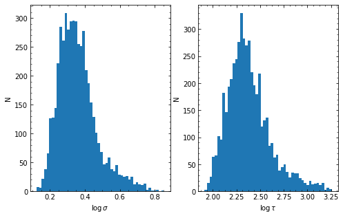
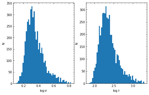
If verbose=True, the posteriors of these parameters \((\log(\sigma_{\rm DRW}), \log(\tau_{\rm DRW}))\) will be shown with histograms of the MCMC samples. Afterwards, JAVELIN will use the median values of these parameters and their uncertainties as priors for the actual JAVELIN fit.

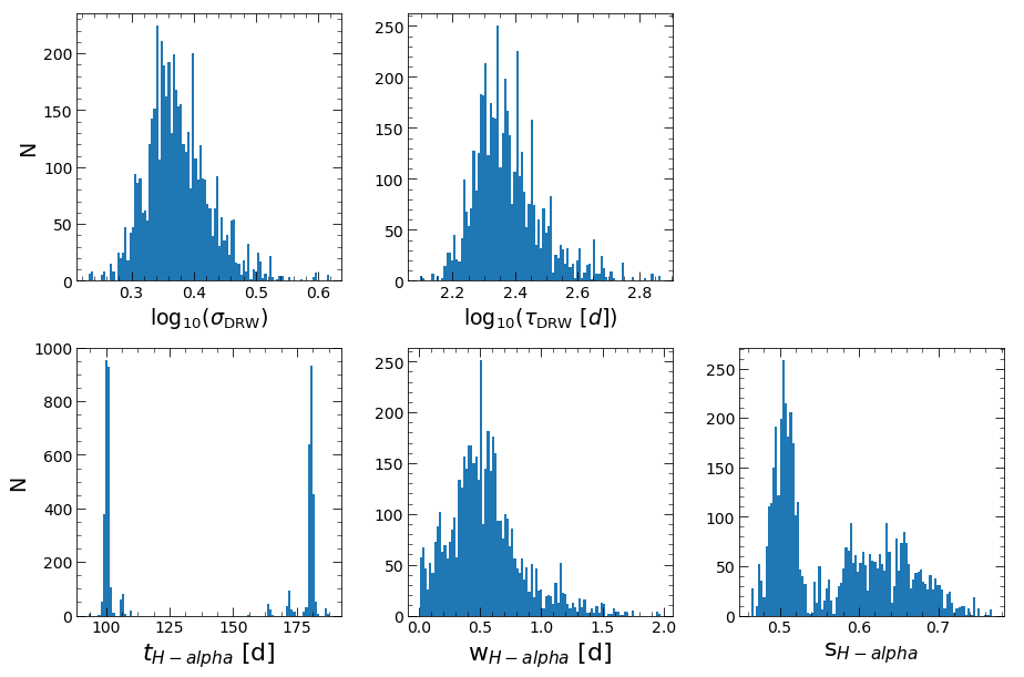
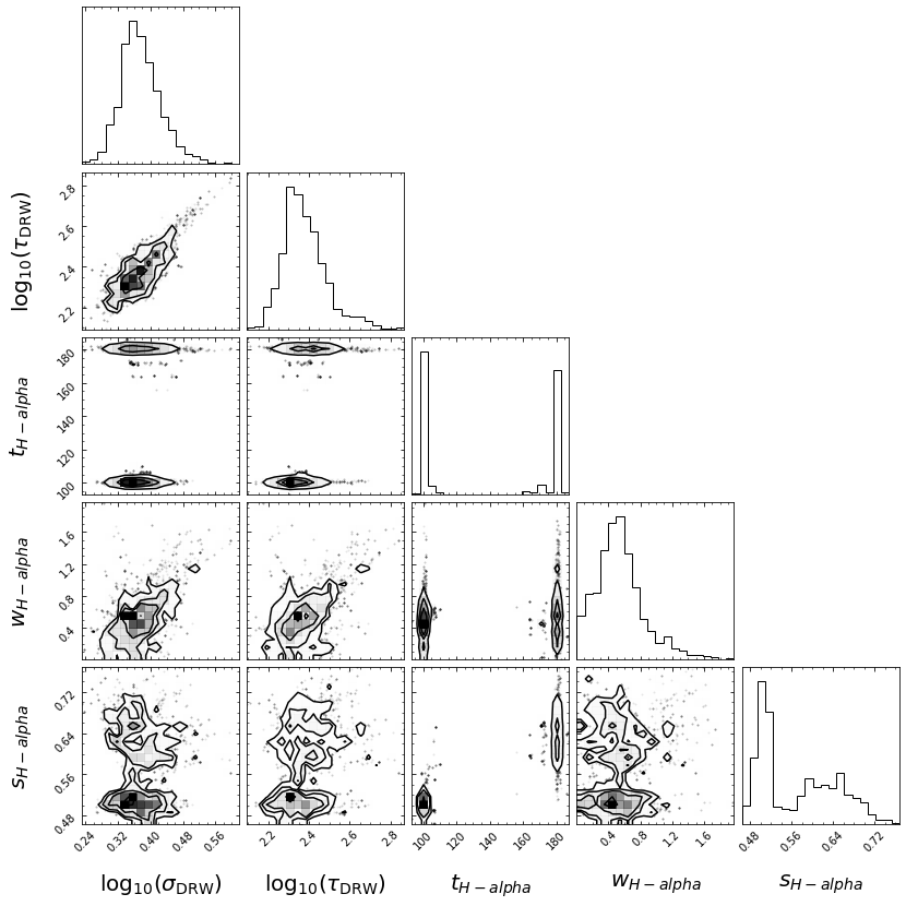
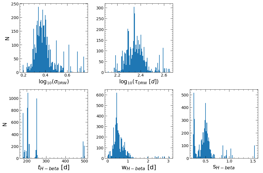
Then, JAVELIN will fit the light curves (all if together=True, and the continuum and each light curve separately if together=False) to the DRW+tophat model. The MCMC samples will be shown in histograms again, and the median values of these distributions will be used as the fit parameters. Additionally, a corner plot will be shown, showing the correlations between the parameters.

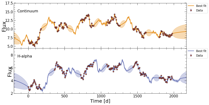
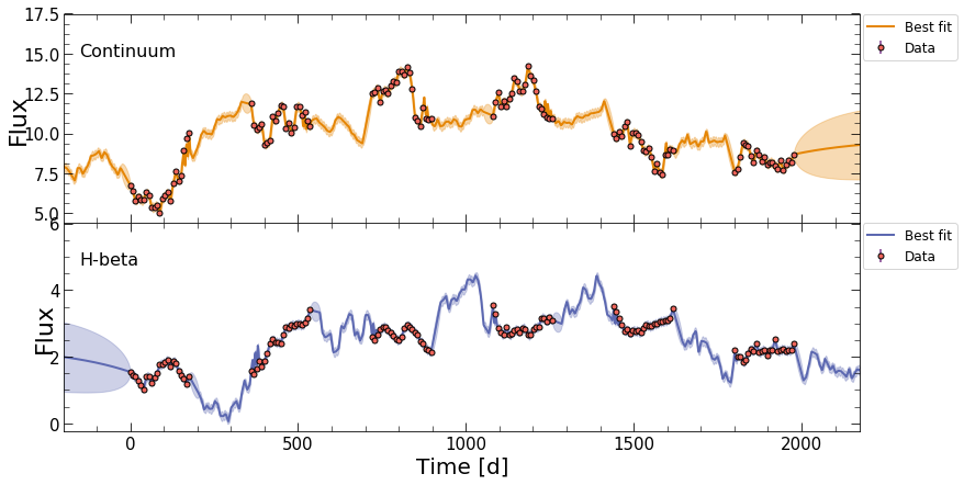
Afterwards, JAVELIN will be used to predict the light curves at a higher cadence, using the best-fit DRW and tophat parameters.

A Simple Example

We’ll use the run from the quickstart example (excluding JAVELIN), and run JAVELIN on all light curves individually:

%matplotlib inline
import pypetal_jav.pipeline as pl

output_dir = 'javelin_output1/'
line_names = ['Continuum', 'H-alpha', 'H-beta']

params = {
    'nwalker': 50,
    'nburn': 50,
    'nchain': 100,
    'lagtobaseline': 0.1,
    'nbin': 100
}

res = pl.run_pipeline( output_dir, line_names,
                 javelin_params=params,
                 verbose=True,
                 plot=True,
                 file_fmt='ascii',
                 lag_bounds=[[0,200],[0,500]])

Running JAVELIN
--------------------
rm_type: spec
lagtobaseline: 0.1
laglimit: [[0, 200], [0, 500]]
fixed: True
p_fix: True
subtract_mean: True
nwalker: 50
nburn: 50
nchain: 100
output_chains: True
output_burn: True
output_logp: True
nbin: 100
metric: med
together: False
--------------------

start burn-in
nburn: 50 nwalkers: 50 --> number of burn-in iterations: 2500
burn-in finished
save burn-in chains to /home/stone28/pypetal/javelin_output1/H-alpha/javelin/burn_cont.txt
start sampling
sampling finished
acceptance fractions for all walkers are
0.76 0.68 0.64 0.61 0.76 0.72 0.71 0.81 0.69 0.70 0.80 0.68 0.65 0.68 0.74 0.73 0.64 0.72 0.72 0.73 0.72 0.76 0.80 0.67 0.81 0.74 0.63 0.75 0.65 0.68 0.70 0.60 0.76 0.73 0.64 0.76 0.74 0.67 0.73 0.73 0.86 0.64 0.68 0.74 0.72 0.69 0.78 0.77 0.73 0.64
save MCMC chains to /home/stone28/pypetal/javelin_output1/H-alpha/javelin/chain_cont.txt
save logp of MCMC chains to /home/stone28/pypetal/javelin_output1/H-alpha/javelin/logp_cont.txt
HPD of sigma
low:    1.806 med    2.201 hig    2.838
HPD of tau
low:  147.070 med  221.858 hig  381.812

run single chain without subdividing matrix
start burn-in
using priors on sigma and tau from continuum fitting
[[  1.806 147.07 ]
 [  2.201 221.858]
 [  2.838 381.812]]
penalize lags longer than 0.10 of the baseline
nburn: 50 nwalkers: 50 --> number of burn-in iterations: 2500
burn-in finished
save burn-in chains to /home/stone28/pypetal/javelin_output1/H-alpha/javelin/burn_rmap.txt
start sampling
sampling finished
acceptance fractions are
0.28 0.31 0.29 0.39 0.41 0.18 0.24 0.26 0.21 0.32 0.28 0.27 0.22 0.16 0.18 0.19 0.25 0.35 0.14 0.19 0.29 0.23 0.17 0.20 0.36 0.29 0.23 0.18 0.27 0.31 0.25 0.25 0.27 0.28 0.23 0.30 0.18 0.24 0.27 0.24 0.23 0.16 0.21 0.34 0.29 0.28 0.37 0.20 0.16 0.26
save MCMC chains to /home/stone28/pypetal/javelin_output1/H-alpha/javelin/chain_rmap.txt
save logp of MCMC chains to /home/stone28/pypetal/javelin_output1/H-alpha/javelin/logp_rmap.txt
HPD of sigma
low:    2.139 med    2.338 hig    2.649
HPD of tau
low:  191.662 med  229.231 hig  296.592
HPD of lag_H-alpha
low:  100.217 med  106.366 hig  180.866
HPD of wid_H-alpha
low:    0.258 med    0.512 hig    0.794
HPD of scale_H-alpha
low:    0.498 med    0.545 hig    0.656

covariance matrix calculated
covariance matrix decomposed and updated by U

start burn-in
nburn: 50 nwalkers: 50 --> number of burn-in iterations: 2500
burn-in finished
save burn-in chains to /home/stone28/pypetal/javelin_output1/H-beta/javelin/burn_cont.txt
start sampling
sampling finished
acceptance fractions for all walkers are
0.64 0.69 0.67 0.70 0.68 0.79 0.69 0.71 0.73 0.69 0.67 0.74 0.75 0.64 0.63 0.73 0.74 0.70 0.78 0.75 0.66 0.78 0.72 0.70 0.78 0.72 0.77 0.68 0.61 0.71 0.70 0.80 0.69 0.68 0.76 0.70 0.68 0.75 0.70 0.73 0.72 0.63 0.75 0.67 0.75 0.66 0.70 0.74 0.70 0.73
save MCMC chains to /home/stone28/pypetal/javelin_output1/H-beta/javelin/chain_cont.txt
save logp of MCMC chains to /home/stone28/pypetal/javelin_output1/H-beta/javelin/logp_cont.txt
HPD of sigma
low:    1.778 med    2.158 hig    2.916
HPD of tau
low:  142.124 med  216.272 hig  402.911

run single chain without subdividing matrix
start burn-in
using priors on sigma and tau from continuum fitting
[[  1.778 142.124]
 [  2.158 216.272]
 [  2.916 402.911]]
penalize lags longer than 0.10 of the baseline
nburn: 50 nwalkers: 50 --> number of burn-in iterations: 2500
burn-in finished
save burn-in chains to /home/stone28/pypetal/javelin_output1/H-beta/javelin/burn_rmap.txt
start sampling
sampling finished
acceptance fractions are
0.01 0.12 0.21 0.09 0.31 0.20 0.14 0.11 0.11 0.14 0.23 0.18 0.02 0.24 0.14 0.22 0.19 0.17 0.14 0.13 0.04 0.15 0.06 0.00 0.21 0.23 0.10 0.26 0.27 0.19 0.14 0.05 0.20 0.07 0.19 0.28 0.15 0.18 0.01 0.06 0.11 0.21 0.15 0.25 0.06 0.27 0.13 0.11 0.11 0.04
save MCMC chains to /home/stone28/pypetal/javelin_output1/H-beta/javelin/chain_rmap.txt
save logp of MCMC chains to /home/stone28/pypetal/javelin_output1/H-beta/javelin/logp_rmap.txt
HPD of sigma
low:    2.091 med    2.377 hig    2.919
HPD of tau
low:  192.244 med  223.118 hig  267.553
HPD of lag_H-beta
low:  186.955 med  204.742 hig  250.994
HPD of wid_H-beta
low:    0.333 med    0.486 hig    0.797
HPD of scale_H-beta
low:    0.262 med    0.482 hig    0.575

WARNING:root:Too few points to create valid contours

covariance matrix calculated
covariance matrix decomposed and updated by U

JAVELIN Output Files

JAVELIN’s output files and figures depend on the input parameters given. If together=True, the subdirectory containing all files/figures will be in output_dir/javelin/. If together=False, there will be a subdirectory for each line in output_dir/(line_name)/javelin/.

The output subdirectory will have he following files, where (name) is the input name of the line:

• burn_cont.txt : The burn-in chains from the MCMC for the initial continuum fit

• chain_cont.txt : The chains from the MCMC for the initial continuum fit

• logp_cont.txt: The log-probability output from the MCMC for the initial continuum fit

• burn_rmap.txt: The burn-in chains from the MCMC for the combined fit

• chain_rmap.txt: The chains from the MCMC fit for the combined fit

• logp_rmap.txt: The log-probability output from the MCMC for the combined fit

• (name)_lc_fits.dat: The predicted light curve using the best-fit JAVELIN parameters. There will be one file for each line.

• javelin_bestfit.pdf: A figure showing the fits to the light curves on top of the input data

• javelin_histogram.pdf: A fgure showing the histograms for the posteriors for each of the JAVELIN parameters

• cont_lcfile.dat: A light curve file for the continuum data in JAVELIN format

• (name)_lcfile.dat: A light curve file foe the line in JAVELIN format. There will be one file for each line.

If fixed is set to None (or all parameters are allowed to vary), a corner plot will also be produced:

• javelin_corner.pdf: A corner plot for all of the JAVELIN parameters

Note

Outputting burn_x.txt, chain_x.txt, and logp_x.txt can be turned off by setting output_burn, output_chain, and output_logp to False in javelin_params

In this case, the output directory will look like this, where the javelin directories for both lines are nearly identical:

quickstart_output/
├── Continuum/
├── H-alpha/
│   └── javelin/
│       ├── burn_cont.txt
│       ├── burn_rmap.txt
│       ├── logp_cont.txt
│       ├── logp_rmap.txt
│       ├── chain_cont.txt
│       ├── chain_rmap.txt
│       ├── continuum_lc_fits.dat
│       ├── H-alpha_lc_fits.dat
│       ├── cont_lcfile.dat
│       ├── tot_lcfile.dat
│       ├── javelin_histogram.pdf
│       ├── javelin_corner.pdf
│       └── javelin_bestfit.pdf
├── H-beta/
│   └── javelin/
├── processed_lcs/
├── pyroa/
├── pyroa_lcs/
└── light_curves/

JAVELIN Output Dict

The JAVELIN module will output a dict containing a variety of data products from pyPetal’s JAVELIN analysis. This dict will be stored in the total output dict under the key javelin_res. If together=False, this will be a list of dict, one for each line.

This output dict will contain the following keys:

• cont_hpd: The highest posterior density (HPD) interval for the initial continuum fit. If both DRW parameters are fixed, this will be None. The first column corresponds to \(\sigma_{\rm DRW}\), and the second corresponds to \(\tau_{\rm DRW}\).

• tau: The list of MCMC samples for \(\tau_{\rm DRW}\).

• sigma: The list of MCMC samples for \(\sigma_{\rm DRW}\).

• tophat_params: The list of MCMC samples for the tophat parameters. There will be \(3\cdot(\rm number \ of \ lines)\) columns, grouped in threes for each line in the following order: (lag, width, scale).

• hpd: The HPD interval for the combined fit. The first column corresponds to \(\sigma_{\rm DRW}\), the second corresponds to \(\tau_{\rm DRW}\), and the rest are the tophat parameters, in the same order as described in tophat_params.

• cont_model: The output javelin.lcmodel object for the initial continuum fit

• rmap_model: The output javelin.lcmodel object for the combined fit

• cont_dat: The continuum light curve in a javelin.LightCurve object

• tot_dat: All light curves (continuum + lines) in a javelin.LightCurve object

• bestfit_model: The JAVELIN fit to the light curves in a javelin.zylc.LightCurve object