The number_component Argument

In the first example we’ve shown for MICA2, we only specified the use of 1 gaussian. However, we can let there be an arbitrary amount of Gaussians/tophats. Let’s try using real data with different amounts of Gaussians:

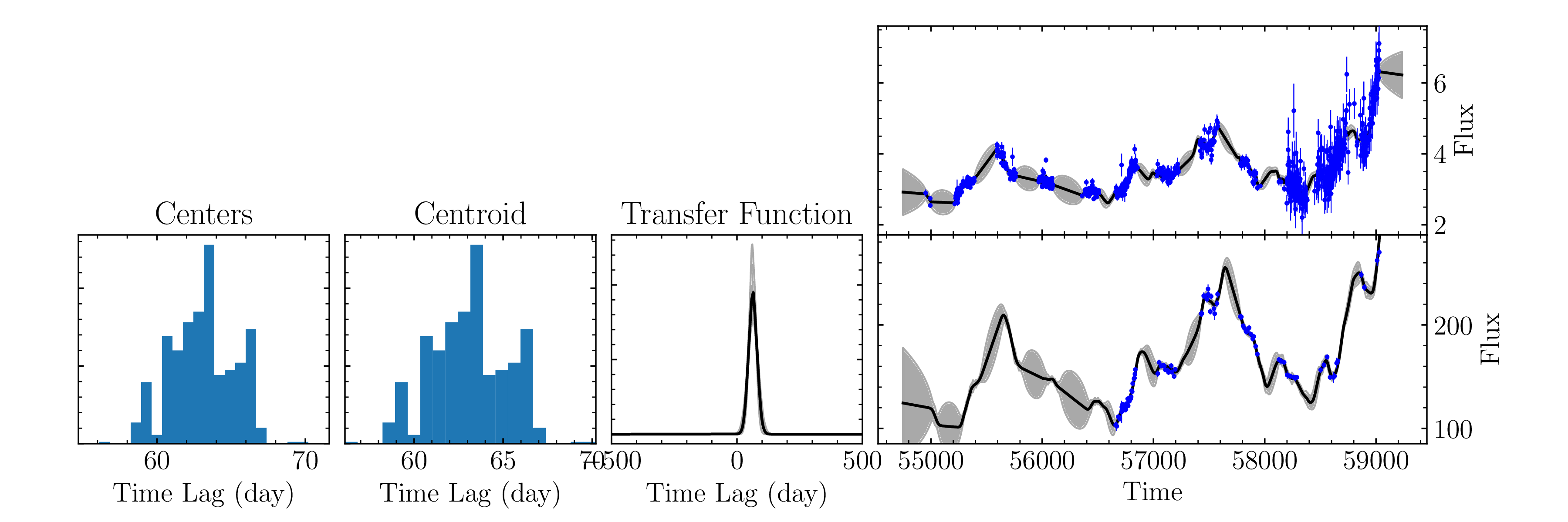
1 Gaussian

%matplotlib inline
import pypetal.pipeline as pl

main_dir = 'pypetal/examples/dat/rm160_'
line_names = ['cont', 'hb']
filenames = [ main_dir + x + '.dat' for x in line_names ]

output_dir = 'mica2_output2a/'




params = {
    'max_num_saves': 2000,
    'no_order': True,
    'number_component': [1,1]
}

res = pl.run_pipeline(output_dir, filenames, line_names,
                      run_mica2=True, mica2_params=params,
                      verbose=True, plot=True, time_unit='d',
                      file_fmt='ascii', lag_bounds=[-500, 500])

Output:

from wand.image import Image as WImage
WImage(filename='mica2_output2a/hb/mica2/data/fig_1.pdf', resolution=300)

2 Gaussians

main_dir = 'pypetal/examples/dat/rm160_'
line_names = ['cont', 'hb']
filenames = [ main_dir + x + '.dat' for x in line_names ]

output_dir = 'mica2_output2b/'




params = {
    'max_num_saves': 2000,
    'no_order': True,
    'number_component': [2,2]
}

res = pl.run_pipeline(output_dir, filenames, line_names,
                      run_mica2=True, mica2_params=params,
                      verbose=True, plot=True, time_unit='d',
                      file_fmt='ascii', lag_bounds=[-500, 500])

Output:

WImage(filename='mica2_output2b/hb/mica2/data/fig_2.pdf', resolution=300)

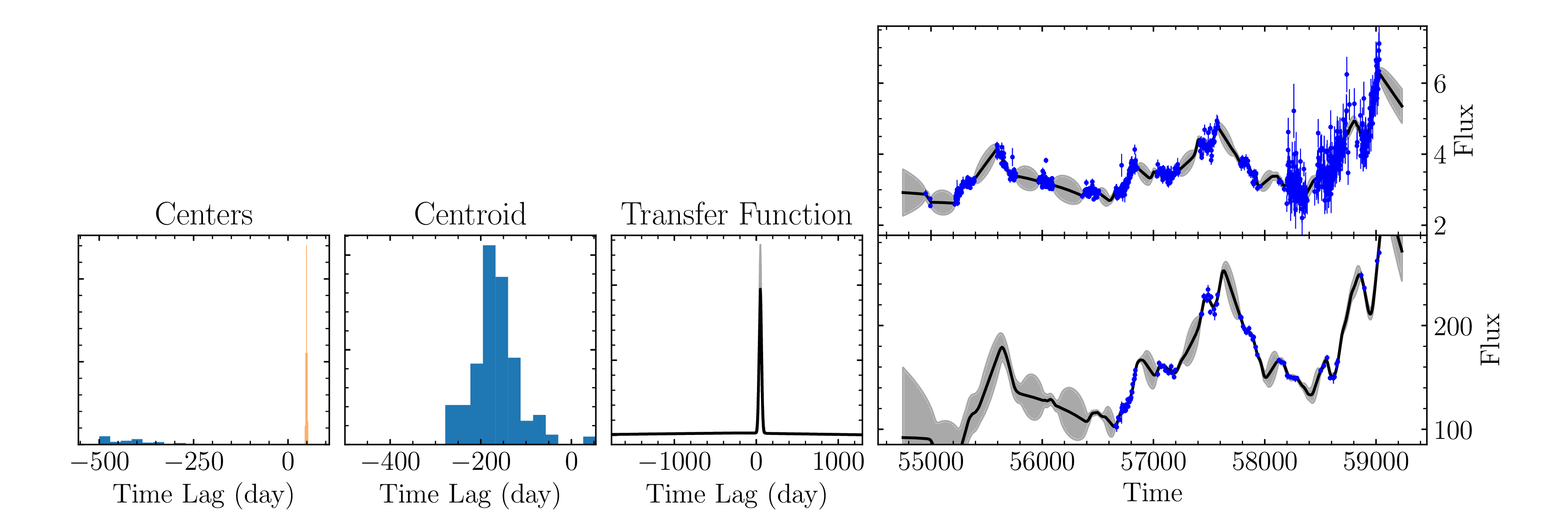
We can see that the fit using one Gaussian is much better than the fit with two in this case. Additionally, the run with two Gaussians took much longer.